Examples
These examples demonstrate how to use the DSPFilter2 operator.
The following example uses the DSPFilter2 operator to produce a moving average of an IBM stock series:
use com.teracloud.streams.timeseries.analysis::DSPFilter2;
composite Main{
  type
    StockSchema = tuple<rstring date, float64 open, float64 high,
            float64 low, float64 close, float64 volume, float64 adjClose>;
  graph
    stream <StockSchema> StockStream = FileSource() {
      param
        file: "stock.csv"; // read some stock data from file
        format: csv;
        initDelay: 1.0f;
    }
    stream <rstring date, float64 open, float64 maOpen> FilteredStockStream = DSPFilter2(StockStream){
      param
        xcoef: {0u:0.2,1u:0.2,2u:0.2,3u:0.2,4u:0.2};  // implement a moving average with lag 2
        ycoef: {0u:1.0}; // output value coefficient is always 1
        inputTimeSeries: Open; // the time series to be filtered
      output
        filteredStockStream:
          maOpen=filteredTimeSeries();  // get the trend value
    }
}
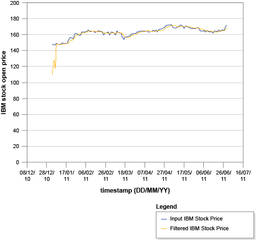
The following graph illustrates how short-term fluctuations in stock prices are smoothed out when you use a DSPFilter2 operator to calculate a moving average:

The following example demonstrates how you can use the DSPFilter2 operator to extract signal components. In particular, a sine wave is separated from a noisy sine wave. Two DSPFilter2 operators are used: the first extracts the sine wave and the second extracts the noise:
// Read the noisy sinewave
stream <float64 time, float64 noisysine> sineStream = FileSource(){
  param
    file: "noisysine.csv";
    format: csv;
    initDelay: 1.0f;
}

// Extract the sine wave by using a low-pass filter
stream <float64 time, float64 noisysine, float64 sine> extractSineStream = DSPFilter2(sineStream){
  param
    xcoef: {0u:0.2,1u:0.2,2u:0.2,3u:0.2,4u:0.2};  // implement a moving average of lag 5 to smooth out th noise and get sinewave
    ycoef: {0u:1.0}; // output value coefficient is just one (this is a FIR filter)
    inputTimeSeries: noisysine;
  output
    extractSineStream:
      sine=filteredTimeSeries(); // get smoothed value, which is the original sine
}

// Now extract the noise by using a high-pass filter.
// The coefficients of the filter are estimated by using an external tool
stream<float64 time, float64 noisysine, float64 sine, float64 noise> extractNoiseStream = DSPFilter2(extractSineStream) {
  param
    xcoef: {0u:0.4328,1u:-1.7314,2u:2.5971,3u:-1.7314,4u:0.4328};
    ycoef: {0u:1.0000,1u:-2.3695,2u:2.3140,3u:-1.0547,4u:0.18740};  // value at 0 is always 1
    inputTimeSeries: noisysine;
  output
    extractNoiseStream:
    noise=filteredTimeSeries();
}

// Write out the result
() as SinkOP3=FileSink(extractNoiseStream){
  param
    file: "decomposedSine.csv";
}
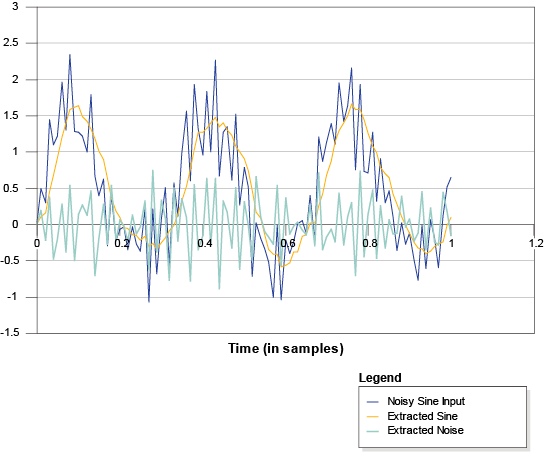
The following graph illustrates the separation of a sine wave from a noisy sine wave:

The figure shows the noisy sine wave, as well as its extracted components: the sine wave and the noise.
The following example shows how the DSPFilter2 operator filters all signals less than 5.0 Hz from the multi dimensional ECG time series data:
use com.teracloud.streams.timeseries.analysis::DSPFilter2;
composite Main {
  type
    ECGRaw = tuple<float64 delay, float64 ts, rstring patientID, list<float64> ECGValue>;
    ECGDerivative = tuple<float64 ts, rstring patientID, list<float64> derivative, list<float64> ECGValue>;
    ECGDerivative2 =  tuple<float64 ts, rstring patientID, list<float64> derivative>;

  graph
    stream<ECGRaw> rawECGStream = FileSource(){
      param
        file : "ts.dat";
        format: csv;
    }

    stream<ECGDerivative> ecgDerivativeStream = DSPFilter2(rawECGStream) {
      param
        filterType: HighPass;       //implement a high-pass filer
        inputTimeSeries: ECGValue;
        cutOffFrequency: 5.0;       // cut off frequency of high-pass filter
        samplingRate: 1000.0;       // sampling rate of the data in Hz
      output
        ecgDerivativeStream: derivative = filteredTimeSeries();
    }

    () as SinkOP = FileSink(ecgDerivativeStream){
      param
        file: "firstOrder.csv";
        format:csv;
    }
}
